Implications of globalization and secular stagnation for monetary policy
The following is a lightly edited transcription of a talk given by Josh Bivens at an AFL-CIO conference on the Implications of Globalization & Secular Stagnation for Monetary Policy.
The central question this presentation is “what are the implications of globalization and secular stagnation for monetary policy?” Let me tell you my final answer first and then I’ll work my way there.
My final answer is that globalization and secular stagnation make a sustained, coordinated fiscal expansion necessary for restoring growth to the global economy. Current politics in both the Unites States and Europe make this impossible in the short run. This means it’s likely to be a long time before we have a decent global economy, and that’s a real problem.
Let’s start out with some definitions. Secular stagnation is a chronic shortfall of aggregate demand that cannot be solved just by lowering short-term interest rates. It is obviously closely related to the problems of the zero lower bound (ZLB) on interest rates—it essentially says that this ZLB problem is not something that needs a one-time burst of policy activism to defeat, but that long-run forces (the rise of inequality, among other things) have lowered the long-term natural rate of interest that is consistent with full employment.
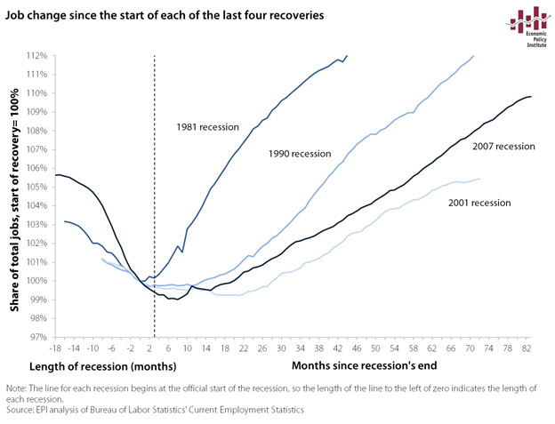
The problem of secular stagnation in the advanced world is actually least pressing in the United States—and yet even here we should certainly be worried about it. We know that there has been a long-run trend towards lower real interest rates in the United States over the past three business cycles. And we know that recovery from the last three recessions has been harder and harder to get going.
Reckoning with secular stagnation requires some serious reorientation on the part of macroeconomic policymaking. For a generation or more, the reigning orthodoxy held that the central problem of macroeconomic stabilization was restraining aggregate demand growth so that it didn’t constantly run ahead of growth in the economy’s growth potential output. The thought was that spending by households, businesses, and government generally was trying to grow faster than what could actually be supplied by the economy’s productive capacity. This meant concretely that the macroeconomic problems to be feared were inflation that was driven by excessive wage growth and rising interest rates. Of course, there were periods when growth in aggregate demand lagged behind growth in potential supply (normal people call these recessions), but it was taken as given that these periods would be short, and recovery would come quickly when monetary policymakers lowered short-term rates a bit. Fiscal policymakers were all but irrelevant in this view of macro policy.
Faith in this quick recovery was even strong in early 2008, when proponents pushing the first stimulus package passed in the Great Recession (the Bush tax rebates) insisted that such a package be targeted, temporary, and timely. Targeted is fine. But temporary and timely really overestimated how rapidly recovery was going to come—and also ruled out some of the most effective stimulus ideas, like infrastructure investment.
Recovery has been defined downward: Actual GDP and estimates of potential GDP in various years, 2008–2015
| Date | 2008 | 2010 | 2012 | 2014 | 2016 | Actual |
|---|---|---|---|---|---|---|
| 2006Q2 | 0 | 0 | 0 | 0 | 0 | 0 |
| 2006Q3 | 0.6849 | 0.6269 | 0.5938 | 0.5998 | 0.6070 | 0.0891 |
| 2006Q4 | 1.3753 | 1.2631 | 1.1943 | 1.2065 | 1.2057 | 0.8725 |
| 2007Q1 | 2.0700 | 1.9094 | 1.8034 | 1.8132 | 1.7846 | 0.9349 |
| 2007Q2 | 2.7704 | 2.5580 | 2.4221 | 2.4405 | 2.3421 | 1.7074 |
| 2007Q3 | 3.4748 | 3.2105 | 3.0398 | 3.0610 | 2.8805 | 2.3914 |
| 2007Q4 | 4.1828 | 3.8630 | 3.6518 | 3.6815 | 3.3963 | 2.7568 |
| 2008Q1 | 4.8941 | 4.5101 | 4.2483 | 4.2813 | 3.8798 | 2.0556 |
| 2008Q2 | 5.6065 | 5.1579 | 4.8400 | 4.8604 | 4.3489 | 2.5621 |
| 2008Q3 | 6.3197 | 5.7926 | 5.4135 | 5.4119 | 4.7940 | 2.0700 |
| 2008Q4 | 7.0333 | 6.4056 | 5.9632 | 5.9428 | 5.2131 | -0.0864 |
| 2009Q1 | 7.7461 | 6.9930 | 6.4772 | 6.4254 | 5.6095 | -1.4709 |
| 2009Q2 | 8.4594 | 7.5393 | 6.9347 | 6.8597 | 5.9572 | -1.6039 |
| 2009Q3 | 9.1729 | 8.0492 | 7.3660 | 7.2665 | 6.2788 | -1.2824 |
| 2009Q4 | 9.8871 | 8.5250 | 7.7777 | 7.6525 | 6.5779 | -0.3269 |
| 2010Q1 | 10.6028 | 8.9628 | 8.1682 | 8.0179 | 6.8502 | 0.1042 |
| 2010Q2 | 11.3185 | 9.3766 | 8.5612 | 8.3833 | 7.1142 | 1.0713 |
| 2010Q3 | 12.0366 | 9.7827 | 8.9579 | 8.7418 | 7.3714 | 1.7540 |
| 2010Q4 | 12.7582 | 10.1934 | 9.3654 | 9.1072 | 7.6279 | 2.3949 |
| 2011Q1 | 13.4843 | 10.6289 | 9.8152 | 9.5002 | 7.9063 | 1.9994 |
| 2011Q2 | 14.2172 | 11.0931 | 10.2809 | 9.9000 | 8.1745 | 2.7417 |
| 2011Q3 | 14.9568 | 11.5867 | 10.7598 | 10.3137 | 8.4495 | 2.9576 |
| 2011Q4 | 15.7028 | 12.1121 | 11.2544 | 10.7411 | 8.7362 | 4.1173 |
| 2012Q1 | 16.4566 | 12.6716 | 11.7467 | 11.1755 | 9.0339 | 4.8075 |
| 2012Q2 | 17.2158 | 13.2598 | 12.2398 | 11.6305 | 9.3637 | 5.2969 |
| 2012Q3 | 17.9789 | 13.8774 | 12.7412 | 12.0855 | 9.7156 | 5.4230 |
| 2012Q4 | 18.7447 | 14.5230 | 13.2533 | 12.5474 | 10.0894 | 5.4470 |
| 2013Q1 | 19.5107 | 15.1894 | 13.7783 | 13.0162 | 10.4995 | 5.9467 |
| 2013Q2 | 20.2771 | 15.8814 | 14.3187 | 13.4850 | 10.9329 | 6.2414 |
| 2013Q3 | 21.0435 | 16.5990 | 14.8759 | 13.9607 | 11.3781 | 7.0242 |
| 2013Q4 | 21.8094 | 17.3383 | 15.4519 | 14.4433 | 11.8300 | 8.0324 |
| 2014Q1 | 22.5747 | 18.1016 | 16.0534 | 14.9328 | 12.2710 | 7.7816 |
| 2014Q2 | 23.3391 | 18.8843 | 16.6756 | 15.4223 | 12.7072 | 8.9920 |
| 2014Q3 | 24.1030 | 19.6801 | 17.3180 | 15.9324 | 13.1420 | 10.1387 |
| 2014Q4 | 24.8665 | 20.4845 | 17.9801 | 16.4564 | 13.5748 | 10.7049 |
| 2015Q1 | 25.6302 | 21.2904 | 18.6614 | 17.0010 | 14.0028 | 10.8824 |
| 2015Q2 | 26.3940 | 22.0948 | 19.3634 | 17.5664 | 14.4273 | 11.9537 |
| 2015Q3 | 27.1591 | 22.8961 | 20.0843 | 18.1524 | 14.8532 | 12.5048 |
| 2015Q4 | 27.9257 | 23.6904 | 20.8233 | 18.7590 | 15.2846 | 12.7865 |
Note: Shaded area denotes recession. Measures of potential output are from forecasts in successive editions of the CBO Budget and Economic Outlook from 2008 to 2016.
Source: Author’s analysis of data from BEA NIPA Table 1.1.6 and the Congressional Budget Office (on potential gross domestic product)
Secular stagnation flips all of this on its head. Generating sufficient demand to pin the economy at full employment now has to be seen as a) difficult and b) the primary task of macro policymakers. Failing to solve the problem of demand then boomerangs back to erode the economy’s potential output as well. The figure here shows successive estimates from 2007 to 2016 of the economy’s potential output.
All of these trends are worse in Japan and Europe. So, this is very worrisome just from a human welfare angle. But it turns out that having most of the advanced world afflicted by secular stagnation also severely blunts the effectiveness of some crucial macro policy tools that could work to restore aggregate demand growth in a closed economy. Let’s run through some of these levers.
Exchange-rate policy
Let’s start with exchange rates. As a macroeconomic tool, the first thing to realize is that first-round effects of exchange rate policy (i.e., before multipliers kick-in) simply redistribute aggregate demand between countries. That’s fine in normal times, but it’s potentially more problematic these days.
Between approximately 2007–2013, there was unambiguous evidence not only that an exchange rate appreciation of the Chinese currency vis-a-vis the U.S. dollar would redistribute aggregate demand from China to the United States, but also that this redistribution would lead to a net increase in aggregate demand globally. The United States was stuck at the ZLB while China was not. A redistribution of aggregate demand from China to the United States would boost the U.S. economy, while China had room to use other macro tools to keep their level of aggregate demand constant.
Even more straightforward, the institutional mechanism keeping this appreciation from happening was really clear-cut—the Chinese government was intervening through huge increases in dollar reserves, keeping the needed appreciation from occurring. The resulting policy solution was pretty clear: stop the mercantilist currency management, and create jobs.
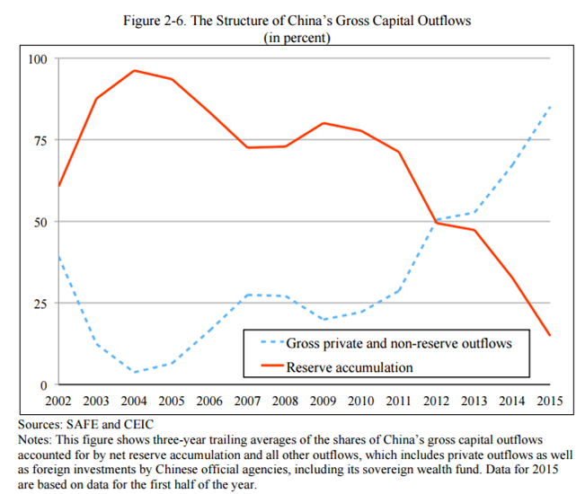
It seems to me that this situation has gotten a bit more complicated recently. There is still lots of money flowing out of China, but more of it in very recent years (or at least looks) looks private, not official.
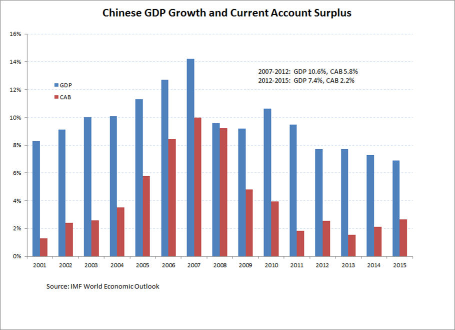
China’s growth also seems to be slowing substantially. And while the Chinese current account surplus has increased in the past year, it was relatively small in 2013 and 2014. In short, the implied benefits of a policy to end official mercantilist currency management seem quite a bit smaller to me today than in 2007-2013.
Let me be really clear on this: we need international agreements that give countries tools to push back on this mercantilist currency management. This management was a big problem for years, and could well be again. The analogy is having a roofless house that lets rain pour down on you during a storm. When the storm is over, it doesn’t make a lot of sense to say “well, it’s not raining any more, so, guess we don’t need to build that roof.”
But, besides this key policy point, I think the prospect for aggregate demand redistribution through exchange-rate adjustment to spur growth in the United States has gotten a bit dimmer in recent years. Having China be able to export aggregate demand to us and yet keep growing strongly was the real hope. And maybe the Chinese slowdown is overblown (people have been calling for it for a long time). But the easy “end currency management and global aggregate demand will grow” solution seems like it’s gotten harder recently .
There is of course one country that is growing well right now, has a very small output gap (if any), and has an enormous current account surplus that could afford to redistribute some aggregate demand to the rest of the world. That country, of course, is Germany. But, this redistribution would be hard to do with exchange rates. About half of their trade surplus is intra-Euro, and, if the Euro appreciated to try to export aggregate demand to the rest of the world, Greece, Spain, and Ireland would suffer.
Monetary policy
So, let’s move on to monetary policy. Only part of the boost from expansionary monetary policy comes from exchange rate depreciation, but, this part is again, aggregate redistribution, and this means that the effectiveness of monetary policy can be partially blunted if some of your major export markets are stuck at the ZLB.
The logic is simple—when we lower rates, part of the aggregate demand expansion comes through more a competitive dollar, leading to a reduction in our trade deficit. If all our trading partners were at full employment, then this would not be a problem. They could accommodate the rising trade deficit through lower rates. But if they’re at the ZLB, this just becomes a redistribution, rather than a net increase, of aggregate demand.
Of course, the United States is not currently talking about expansionary monetary policy, we’re instead talking about monetary policy restraint. But globalization and secular stagnation are relevant here as well. The boost to the dollar stemming from higher U.S. rates will redistribute demand from the United States towards Europe and Japan. This could be useful, or dangerous.
If the United States was genuinely at full employment and if all that Japan and the EU needed was a small nudge, one could argue that a U.S. rate increase and resulting dollar appreciation could pull them out of their funk.
But if instead they’re sunk deep into secular stagnation and require a lot more macro support than could plausibly be transferred via a dollar appreciation, and if the U.S. economy is not firmly at full employment and actually has slack and could sputter soon, then this exchange rate linkage could mean that they just pull us back down into stagnation as a result of aggregate demand redistribution. This is why some authors have recently described secular stagnation as a potentially “contagious malady.”
Further, the size of the dollar drag on recovery following a U.S. rate increase will depend on which scenario is likely to hold. If everybody thinks the EU and Japan just need a nudge, then redistributing some aggregate demand to them will pull them out of their liquidity trap, and rates in the EU and Japan will be expected to move closer to U.S. rates before long, and the dollar’s rise following a rate increase will be small.
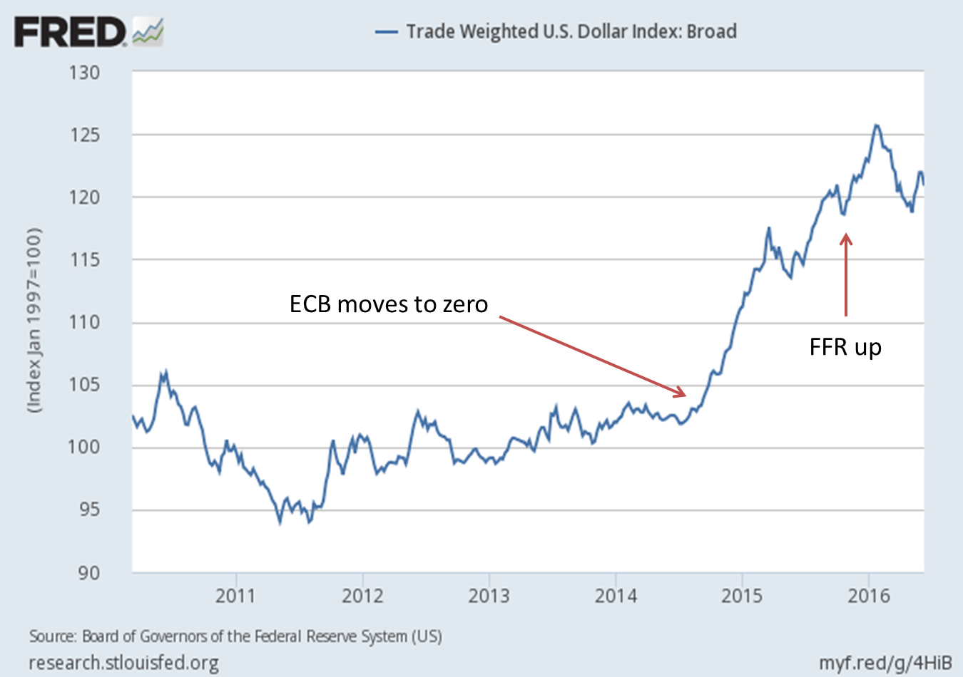
However, if everybody instead thinks that they’re sunk deep, then expectations of a recovery-driven rise in EU and Japan rates will not be there, and the response to the gap opened up by a US interest rate increase will be large. This means it’s going to be very hard to “tap” the brakes going forward—every time you put your foot on the brake pedal will slow the car more than you likely think. And recent evidence shows the dollar is pretty sensitive to differences in rates between the United States and other advanced countries.
Fiscal policy
So where are we now? The prospect of boosting global demand simply through figuring out how to make China stop mercantilist currency management has worsened in recent years. Monetary expansion is blunted partially through the ZLB position of trading partners. Monetary tightening just shouldn’t be done, and will be more painful now than generally because of the ZLB position of our trading partners.
What to do? The answer is, of course, as easy economically as it is remote politically: a substantial, coordinated fiscal expansion. Fiscal policy is pure aggregate demand generation, not redistribution. Its intl spillovers are positive, not negative.
There is no evidence at all that large countries are out of fiscal space. The United States and Germany, in particular, have all the room in the world to undertake a fiscal expansion.
Fiscal austerity explains the slow recovery: Change in per capita government spending over past six business cycles
| Quarters before and after recession’s trough (trough = 0) | 1975q1 | 1980q3 | 1982q4 | 1991q1 | 2001q4 | 2009q2 |
|---|---|---|---|---|---|---|
| -6 | 90.83817 | |||||
| -5 | 94.14608 | 96.46779 | 91.33168 | |||
| -4 | 95.58078 | 96.72548 | 97.80345 | |||
| -3 | 96.75442 | 96.51523 | 96.35624 | 94.05089 | ||
| -2 | 97.19567 | 99.12375 | 97.21731 | 98.09825 | 98.14218 | 94.4813 |
| -1 | 97.81814 | 98.81721 | 98.26435 | 98.92533 | 97.98324 | 96.68474 |
| 0 | 100 | 100 | 100 | 100 | 100 | 100 |
| 1 | 101.4549 | 99.26806 | 100.3829 | 100.7468 | 101.5275 | 99.84022 |
| 2 | 102.2914 | 99.73443 | 100.9558 | 100.4456 | 102.3723 | 99.50632 |
| 3 | 102.7309 | 99.32341 | 101.005 | 100.9653 | 102.8023 | 100.7222 |
| 4 | 103.1591 | 99.98405 | 99.79553 | 102.3054 | 103.3013 | 101.0192 |
| 5 | 101.5995 | 100.4771 | 102.4831 | 103.1351 | 101.1242 | |
| 6 | 101.6376 | 101.715 | 102.7714 | 104.3665 | 100.3429 | |
| 7 | 101.3162 | 102.037 | 102.2554 | 104.5556 | 98.8815 | |
| 8 | 101.6571 | 103.485 | 101.9195 | 104.6451 | 98.15728 | |
| 9 | 101.7618 | 104.602 | 101.724 | 105.4192 | 97.23711 | |
| 10 | 101.9609 | 106.0107 | 102.011 | 105.8382 | 96.8626 | |
| 11 | 101.5335 | 107.6073 | 101.868 | 105.804 | 95.92456 | |
| 12 | 101.3926 | 107.6288 | 101.2959 | 105.4445 | 95.78462 | |
| 13 | 102.7633 | 108.7749 | 101.4328 | 106.1767 | 95.40432 | |
| 14 | 103.7289 | 110.4932 | 102.1325 | 106.3521 | 94.83228 | |
| 15 | 103.9792 | 112.3029 | 101.9209 | 106.5289 | 94.20283 | |
| 16 | 103.0743 | 111.6476 | 102.6275 | 106.0185 | 93.88481 | |
| 17 | 103.3799 | 112.0741 | 102.8173 | 107.5423 | 93.60793 | |
| 18 | 104.385 | 112.6221 | 102.3836 | 107.6773 | 93.04602 | |
| 19 | 104.6642 | 112.3952 | 101.1486 | 107.8776 | 93.22673 | |
| 20 | 105.8042 | 113.0807 | 101.9359 | 108.2144 | 93.61573 | |
| 21 | 113.3476 | 103.2437 | 109.1187 | 94.26683 | ||
| 22 | 113.3408 | 102.7047 | 109.0787 | 94.17814 | ||
| 23 | 113.108 | 102.7598 | 109.5846 | 95.13453 | ||
| 24 | 114.405 | 103.1194 | 109.8789 | 95.48556 | ||
| 25 | 114.9973 | 103.4402 | 95.77813 |
Note: For total government spending, we deflated government consumption and investment expenditures with the NIPA price deflator. Government transfer payments were deflated with the price deflator for personal consumption expenditures. This figure includes state and local government spending. We agree that it is appropriate to include this spending in a measure of the federal government's failure to combat austerity in the current recovery. Only the federal government has the significant ability to run deficits during recessions, and historically many federal efforts to combat recessions and spur recovery have involved giving aid to state and local governments to spend.
Source: Author’s analysis of data from Tables 1.1.4, 3.1, and 3.9.4 from the National Income and Product Accounts (NIPA) of the Bureau of Economic Analysis (BEA)
It’s not like we’re even asking for a radical fiscal program—just a reversal of the radical fiscal austerity of recent years would do it. But if we had simply spent the way we did during the Reagan recovery, we’d have been at full employment long ago and the Fed could’ve hiked significantly by now.
There’s been a bit of a boomlet in proposals for infrastructure during the presidential primary season—Clinton, Sanders, and Trump have all said nice words about investing in public works. This should be encouraged. And some of these candidates have even put some plans on paper and called for significant amounts. This should really be encouraged. Who knows, maybe even the DC Metro could become reliable and safe again.
Enjoyed this post?
Sign up for EPI's newsletter so you never miss our research and insights on ways to make the economy work better for everyone.